FEA of 3D printed part
In additive manufacturing, it is very important to know how the materials behave under different conditions. Obviously, talking about the behavior of materials does not mean just the filament itself but also the part that is made using that filament. It is obvious that changing processing settings can impact the behavior of any shape. This is not only because of the anisotropic properties of materials and inhomogeneous geometry, but also because of the combination of processing parameters, thermal behaviors, and consolidation. All these impact how the final product acts. This fact makes the simulation of material behavior necessary and very important.
Different software can help us simulate the materials’ behaviors, but all that software has limitations when it comes to simulating the behavior of polymer materials and layered geometries under a variety of conditions.
Finite element analysis can be useful in the industrial field if it can give similar results with a minimum error compared to the real world.
Of course, in the field of additive manufacturing, the best results can be achieved using layered geometry, but modelling layered geometry and implementing the different characteristics of this geometry into the software is very difficult. One of these characteristics is layer adhesion. Layer adhesion means the bonding between each layer and requires that the printing layer and the previous layer melt together. In one product, the adhesion between one layer and the other can be different than in the other. This can be because of temperature differences or inaccurate printing speed.
So, at this moment, it is not possible to implement all conditions into the software. This is because FEA tools were developed to predict the behaviour of solid materials and they do not work well with additive manufactured parts.
Having discussed the limitations of FEA tools, they can still be usable if they can predict the results with some acceptable error.
In this chapter, we will try to study the difference between the results of the analysis in the FE tool and the real world to see if these methods can predict accurate behaviour or not.
The FEA software that will be used is ANSYS.
Ansys is a general-purpose, finite-element modeling package for numerically solving a wide variety of mechanical problems. These problems include static/dynamic, structural analysis, heat transfer, and fluid problems, as well as acoustic and electromagnetic problems.
The goal of these analyses first is to obtain the maximum torque that the model can withstand. Or maximum torque before elastic deformation. Secondly, the angular deformation of the central disk due to increasing of the torque This deformation will occur in the plastic region. We need to know the plastic behavior and properties of a material.
1.1 Defining the geometry
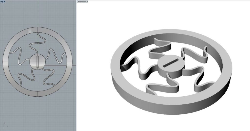
Figure 1: Geometry
The first step is to define the geometry. The geometry which is used here is demonstrated in figure 32. It is a rim-like shape with very thin spokes that connect the outer rim to the centre disk.
The geometry which is analysed in Ansys is solid, which means it does not have the characteristics of a layered model. The reason for this is the limitations of Ansys and, generally, FEA. We talked about it in the previous section.
The spokes of the rim are very narrow. In fact, they are made only with one path of deposited material. It is because we tried to make the 3D printed geometry behave similar to a solid one as much as possible.
In other words, because modelling and analysing layered geometry in FEA is not feasible, we made layered geometry work as if it were solid. In this way, we can get more accurate results and the behavior of the simulated part will be closer to the real world.
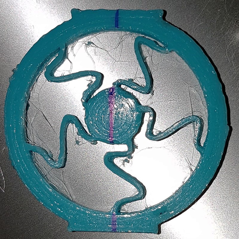
Figure 2: 3d printed Rim using PLA as a material.
The real 3d printed geometry is shown on the figure 2. As it is observable only one path of PLA deposited for creating the spokes.
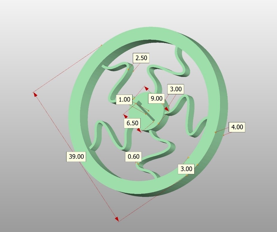
Figure 3: Dimensions of the geometry.
The dimensions of this geometry are shown in figure 3.
1.2 Defining material
After importing the geometry into the Ansys, next step is to define the material.
They are lots of materials on market and in Ansys library with similar properties that can be useable for this work. But it should be considered that even a small variation in material properties can lead to different results.
The material which is used for this experiment is PLA made by manufacturer Filamentum.
The properties of material are showed in figure 4.
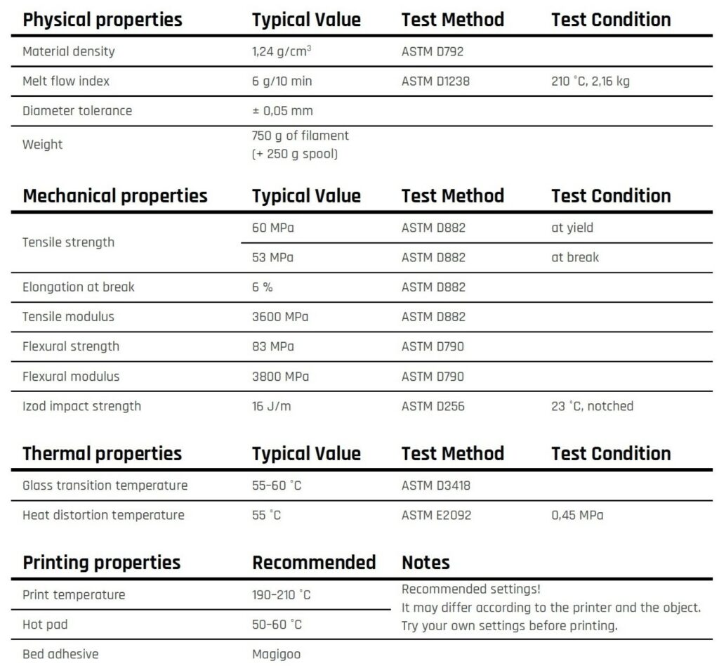
Figure 4: Filamentum PLA datasheet.[21]
One problem here is that the filament datasheet only includes material parameters in the elastic area. However, the plastic characteristics of the material are also required for modeling plastic deformation. Many research have been conducted on the behavior of PLA after yield stress. The values used in this study are taken from the strain stress diagram of this research. [22].
The Poisson ratio is 0.35.
Plastic properties and bilinear isotropic hardening properties are as below.
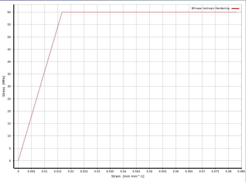
Figure 5: bilinear isotropic hardening
1.3 Meshing the geometry
After implementing the material properties into the material library of Ansys next step is to Mesh the geometry.
Meshing is one of the most important steps in performing an accurate simulation using FEA. A mesh is made up of elements which contain nodes (coordinate locations in space that can vary by element type) that represent the shape of the geometry. An FEA solver cannot easily work with irregular shapes, but it is much happier with common shapes like cubes. Meshing is the process of turning irregular shapes into more recognizable volumes called “elements.”
In general, there are two kinds of meshing procedures. We are referring to 3D models for these purposes:
Tetrahedal element meshing or “tet”
Hexahedral element meshing or “hex”
At lower element counts, hex or “brick” elements produce more accurate results than tet elements. Tet components may be the best solution for complicated geometry.
The size of the mesh is very important in FEA, if the size of the meshes decrease, more accurate results can be achieved but there is limitation such as processing time.
Here the Tetrahedal meshing is used with the size of 0.5mm
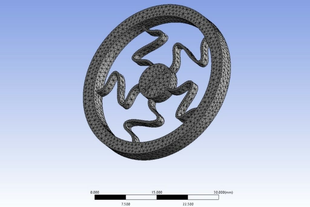
Figure 6: Meshed geometry
Next step is to define boundary conditions, as the goal is the deformation of central disk. The outer ring must be fixed and a torque must be added to central disk in order to rotate it. In order to simulate as close as possible to laboratory test, the torque is added to 2 parallel inner faces which is noticeable in the figure 6.
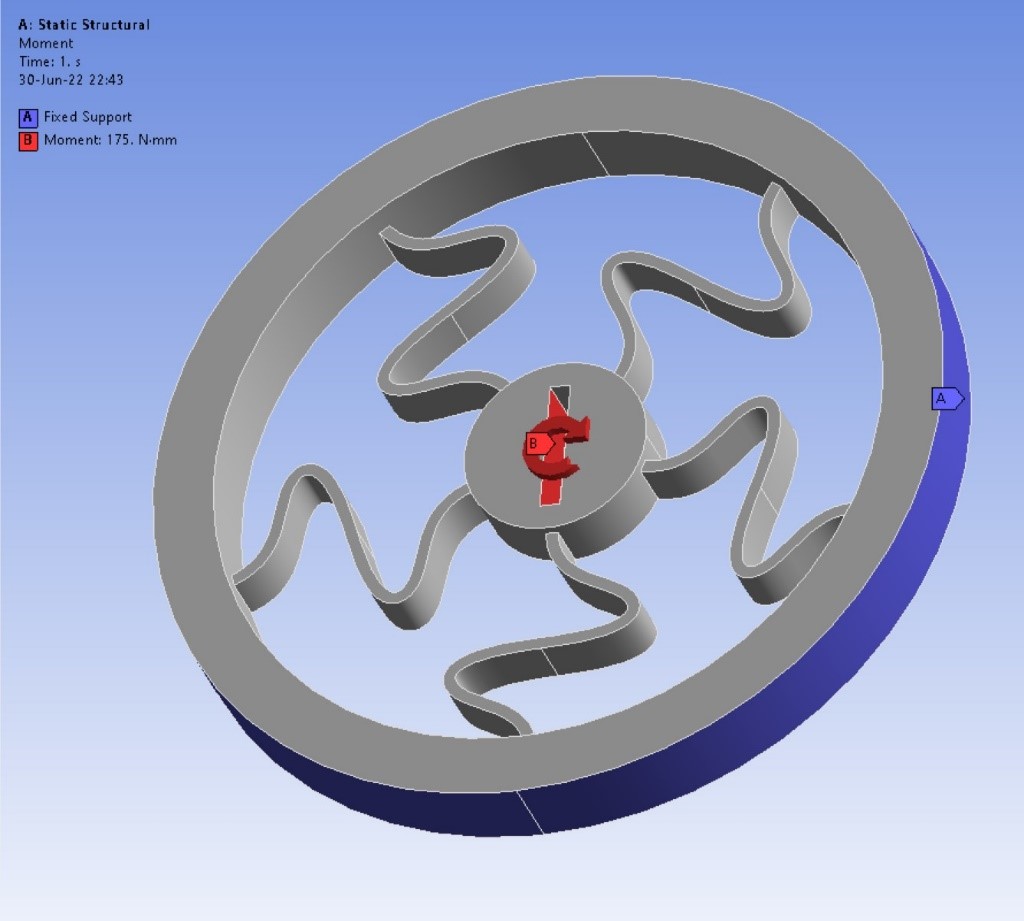
Figure 7: Boundary conditions
The key here is the plastic deformation, normally when we do analysis we want to stay in elastic region, in order not to fail it is important to stay in elastic region. In this case we will explore the plastic region, as well as the unloading scenario. So, we will have some residual strain and deformation after loading and unloading the moment.
Next step is to find the amount of torque which model can withstand or the maximum torque at yield point.
By applying different amounts for moment and reading the maximum stress in results section we can find the maximum torque.
We know that the Yield stress of the material is 60MPa, so we change the value of torque until we reach the 60MPa. This amount is 81Nmm. It means if we apply more than 81nmm the model will permanently deform.
Figure 8. Demonstrates the application of moment to central disk in 3 steps.
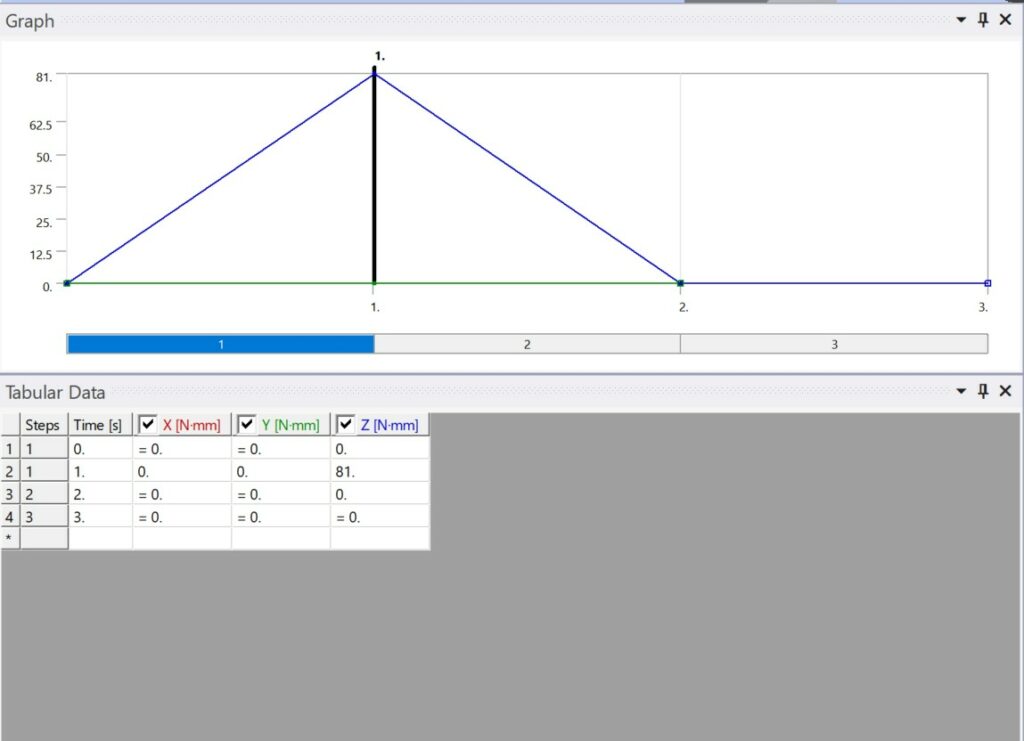
Figure 8. Application of moment.
Figure 9. Shows corresponding stress which is 59.9MPa. And it is in the connection section of spokes to inner disk. It is observable that after unloading the torque in step 2 the amount of stress goes to 0. It means, no residual stress remains in the part.
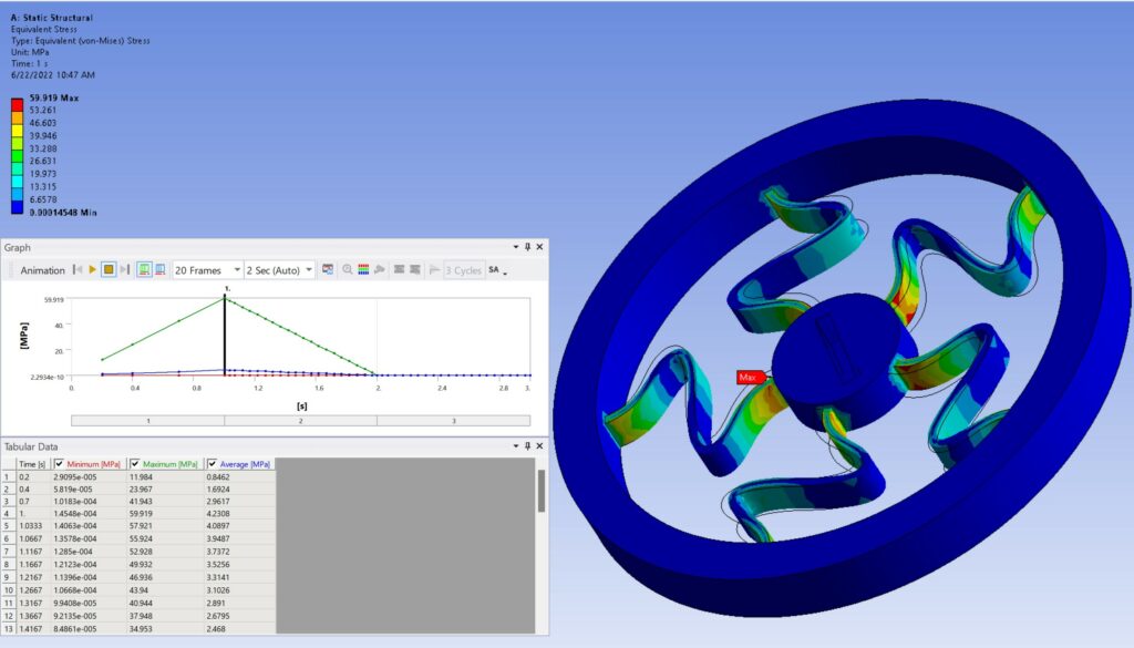
Figure 9: Stress at Yield due to applying of 81nmm torque.
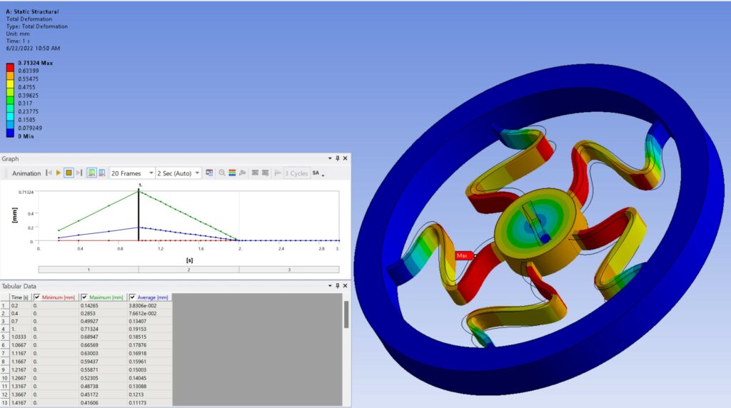
Figure 10: Elastic deformation at Yield (60MPa)
The amount of deformation at yield point is about 0.71mm, this is elastic defamation. It means after unloading the moment, the disk will return to its original position. This amount for angular elastic defamation of central disk is about 7.5 degrees.
Measuring the average rotation of the disk is not available in Ansys results and it needs to be done by use of Remote Point and two ABDL commands.
Ansys parametric design language (APDL) is a scripting language that is used to communicate with the Ansys Mechanical program. It is routinely used in performing parametric design analysis, automating workflows, or even in developing vertical applications for industry-specific problems.
The remote point associated with any point or node or line on the disk and the rotation of the pilot node at the remote point can be measured by APDL commands.
The command:
“Measure_Pilot=_npilot”
used for recording the node number at remote point and the command “my_rotz=ROTZ(Measure_Pilot)*57.29577951”
is used to measure the rotation of the node in degrees. [23]
1.4 Deforming the model
After determining the maximum torque and elastic deformation, the following step is to increase the torque and measure the permanent deformation of the central disk.
To distort the model, the torque was raised to 190nmm. We applied the torque in three stages once more. Figure 11 illustrates the torque application processes, which include loading and unloading.
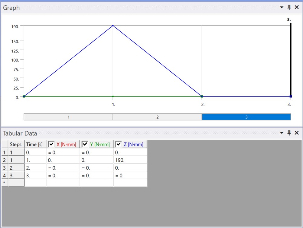
Figure 11: Applying torque in order to deform the geometry.
Corresponding Stress shows in figure 12. As expected, the maximum stress hits the amount of 85MPa. It is far beyond 60MPa which is yield strength. So that confirms that the part is failed and plastic deformation happened.
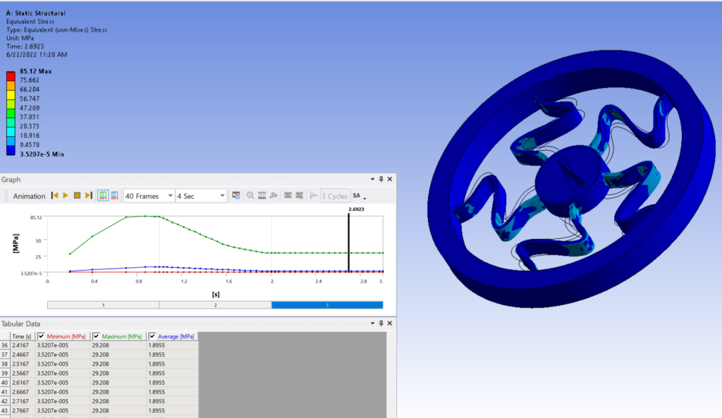
Figure 12: Maximum and residual stress at 190nmm Torque.
The residual stress is equal to 29Mp.
Exploring the total deformation, it is observable from figure 13. That the model starts to deform immediately after applying the torque. The maximum of this deformation is occurred at second 1, where the maximum of 190nmm torque was applied. This deformation is equal to 2.87mm. By unloading the torque, the disk starts to go back to its original shape. At second 2 the deformation of 1.57mm remains in the model which is plastic deformation. Again, the max deformation is in the connected section of spokes to inner disk. By looking closer to spokes it is obvious how they failed and deformed.
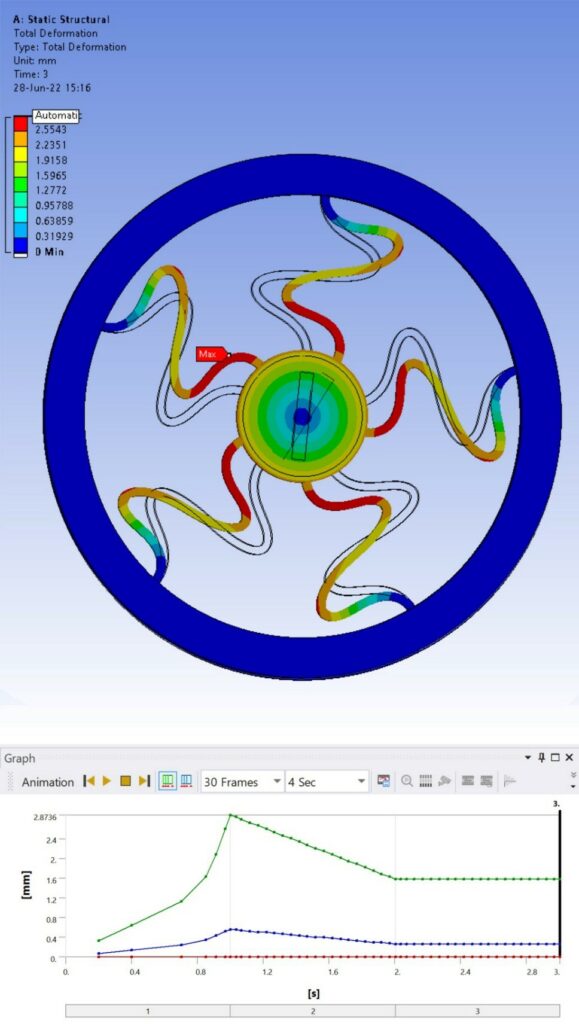
Figure 13: Total deformation.
Obtaining information from APDL Command shows that the final plastic deformation of the inner disk is 17.928 degree to its original position for 190nmm torque.
If we increase the torque the angle of deformation will be increase as well, at about 222nmm we reach the total deformation of 32 degree, which is equal to the deformation of experimented part.
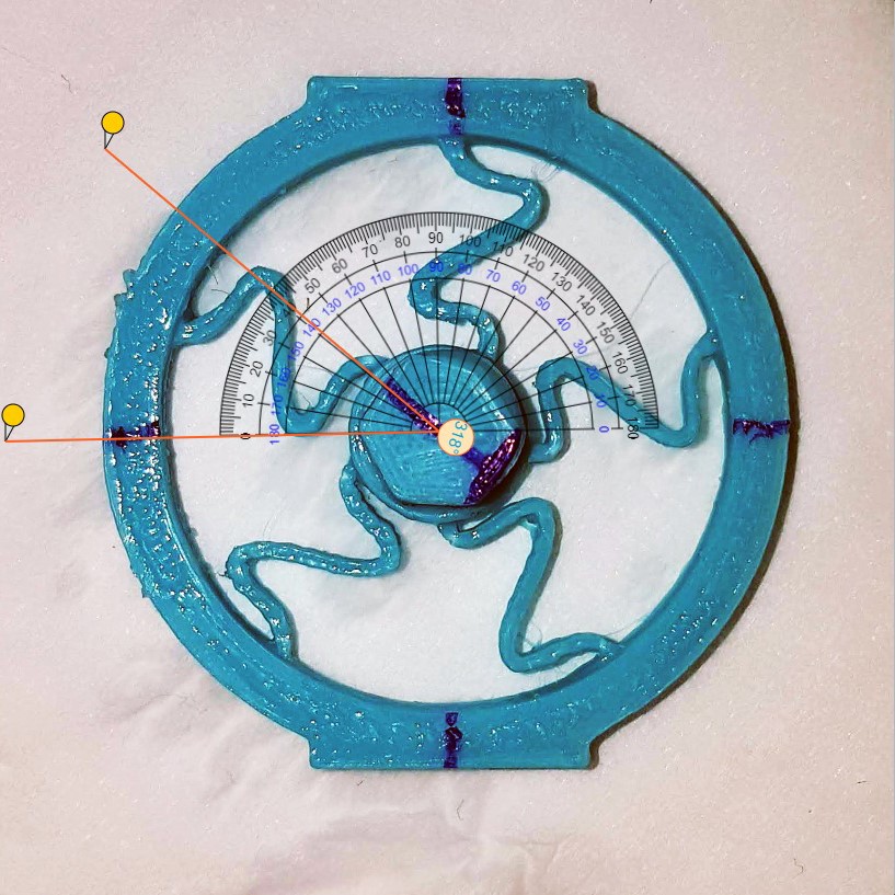
Figure 14: Deformed geometry.
1.5 Comparing simulation and experimental results
The next step is to compare simulation results with experimental results.
In lab by applying 200nmm the inner disk angular deformation was about 32 degree and in Ansys simulation for 32-degree angular deformation we applied 222nmm torque which is very close to experimental data. This was about the angular deformation. Comparing spoke shapes and warpage is also helpful.
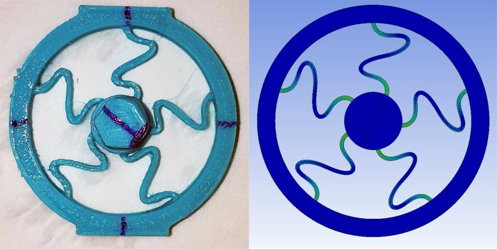
Figure 15: Shape of deformation.
It is clear from comparing the deformation of shapes in figure 46 that the overall deformation forms are relatively comparable. By overlapping 2 photos on figure 47, the differences are perceptible.
The simulated photo demonstrates that the deformation is completely symmetric. This is due to the symmetry of the material form and model we used. The geometry is solid and does not have any material layers. Another possible explanation is boundary conditions. In Ansys we used a fixture for fixing the outer ring and this was distributed to every element of the outer ring.
The outcome of the experimental deformation of the component, on the other hand, is not symmetric. Anisotropic material and layered geometry, residual stress and strain in printed part are possible explanations. The boundary conditions may be the second most important cause. Another cause of this asymmetrical deformation might be the printing processing parameters.
Figure 16 shows that, despite the fact that the deformation of the inner disks are quite close, but the shape of the spokes is not precisely the same, spoke number 4 overlaps but the other spokes do not.
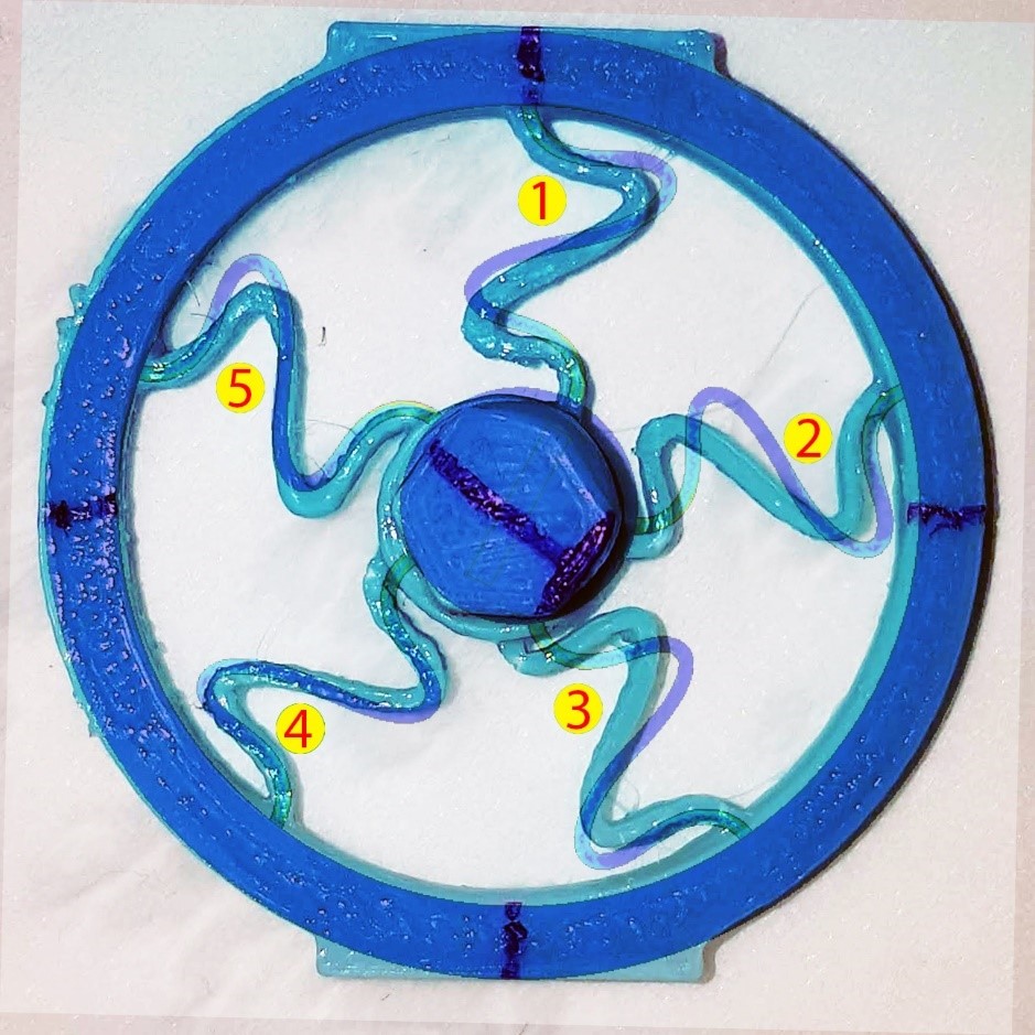
Figure 16: Overlapped photos
1.6 Comparing results with SolidWorks simulation
Next is to see how is the results using other finite element analyses software, here the software that used is SolidWorks simulation.
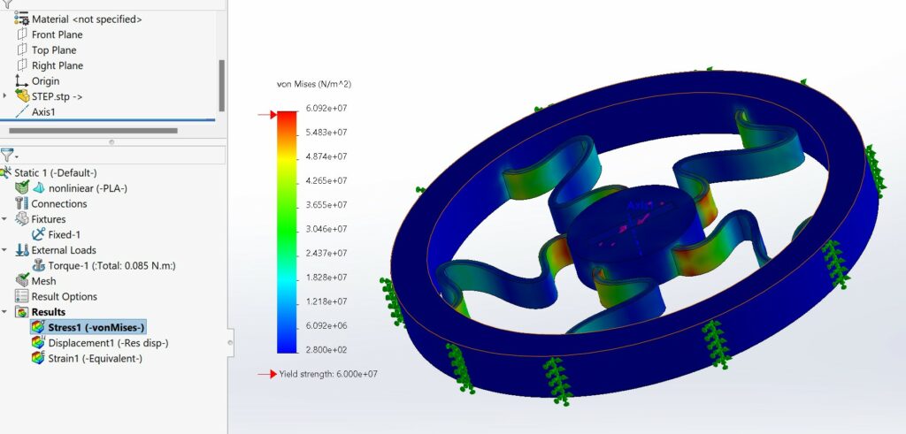
By defining the material and boundary conditions and solving the model for various applied torques, results are obtained as below.
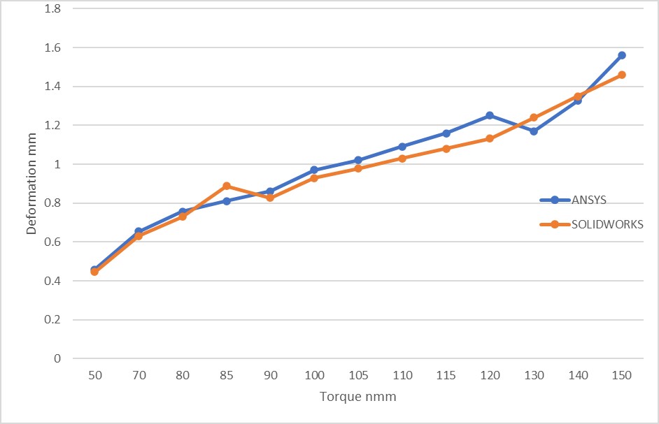
Figure 17: Comparison of 2 software in terms of deformation by increasing applied torque.
Figure 18, shows the similar comparison for stress; as previously discussed, in Ansys, yield stress occurs at 81nmm of applied torque; in SolidWorks, this quantity is around 85nmm. It is also clear that as torque is increased, total stress increases in both programs, but more rapidly in SolidWorks. Unfortunately, as the torque was increased further, the SolidWorks results did not converge, therefore the comparison was terminated at 150nmm.
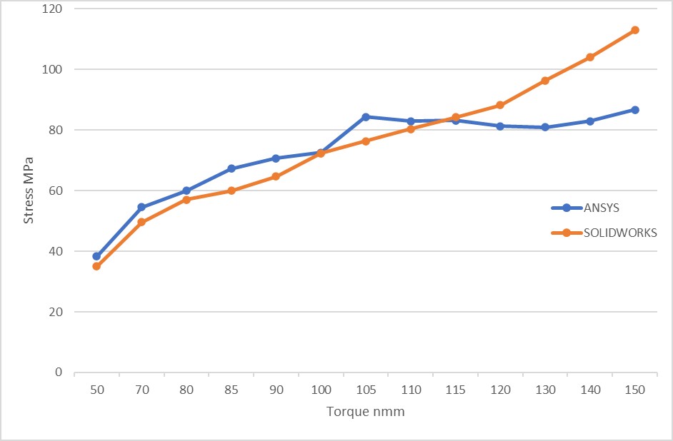
Figure 18: comparison of 2 software in terms of stress by increasing applied torque.
The variation in maximum stress findings between both software is due to their varied behavior with nonlinear systems.
Ansys results are more accurate when it comes to nonlinear analysis. Of course, SolidWorks excels in modelling geometry.
This article was a part of Behrad mostafaee’s master’s thesis.